Ask two imaging scientists to measure the same GFP-labeled cell line on two different widefield systems in the same corridor, and you will frequently obtain mean nuclear intensities that differ by 20 to 35%. The cells are identical. The antibody lot is the same. The protocol was written by the same person. Yet the numbers do not agree — and the disagreement is large enough to change a biological conclusion.
This is not an unusual situation. It is the default state of fluorescence microscopy. The question is not whether inter-instrument variability exists; it is whether your analysis pipeline accounts for it before you draw quantitative conclusions.
The Three Layers of Instrument-Dependent Variability
Fluorescence intensity variability between instruments comes from at least three independent sources, each of which can act alone or compound with the others.
Optical Sources
The transmission efficiency of the excitation and emission light path varies substantially across instruments of the same model, let alone across manufacturers. Dichroic mirrors age and shift their cut-on wavelengths. Objective lens coatings differ in their anti-reflection properties. Filter cubes with nominally identical bandpass specifications can have peak transmission values that differ by 5 to 15% between production batches. A 40x/1.3 NA oil objective on one instrument is not optically identical to a 40x/1.3 NA oil objective on another instrument, even if both are listed as the same part number.
Laser power at the sample plane is a particularly under-appreciated source of variance in confocal systems. Fiber coupling efficiency degrades over time at a rate that depends on alignment history and usage patterns. Two laser lines listed at 10 mW at the fiber output may deliver 6 and 8.5 mW respectively at the objective back aperture after typical field usage of 18 to 24 months.
Electronic and Detector Sources
Camera-based systems introduce gain, offset, and read noise profiles that are specific to the individual sensor. sCMOS sensors have per-pixel gain variation that must be characterized from the actual camera in use, not from a representative unit. Even two sensors from the same production run will have slightly different fixed-pattern noise profiles and slightly different quantum efficiency curves across the visible spectrum.
PMT-based confocal detectors are sensitive to detector gain drift as the tube ages, as well as to temperature fluctuations in the detector housing. Gain calibration procedures exist for these systems, but they are not uniformly performed — and gain settings are rarely documented with sufficient precision in methods sections of published papers.
Software and Acquisition Parameter Sources
This is the layer that most researchers underestimate. Identical hardware can produce different quantitative results depending on how acquisition software scales 12-bit or 16-bit raw sensor data to the stored TIFF or proprietary file. Some acquisition packages apply a default display stretch that also affects the stored data. Others apply a default background offset. The difference between "raw counts" and "display counts" in a .czi or .lif file is not always clearly exposed to the end user.
Equally important: identical camera exposure time on two systems with different illumination intensities at the sample plane will produce non-comparable intensity values. This seems obvious, but many multi-site studies use "the same exposure time" as a proxy for "the same imaging conditions" — a substitution that conflates acquisition parameters with the physical quantity being measured.
A Concrete Scenario: The Same Assay, Two Cities
Consider a typical scenario: an early-stage European biotech running a phenotypic cell health assay across two imaging sites — their own Leica DMi8 widefield system in-house and a Nikon Ti2 system at a collaborating academic core facility. Both sites use the same fixed-cell protocol, DAPI nuclear stain, and a cytoplasmic marker in the GFP channel. Both teams capture 20x images with nominally matched exposure settings.
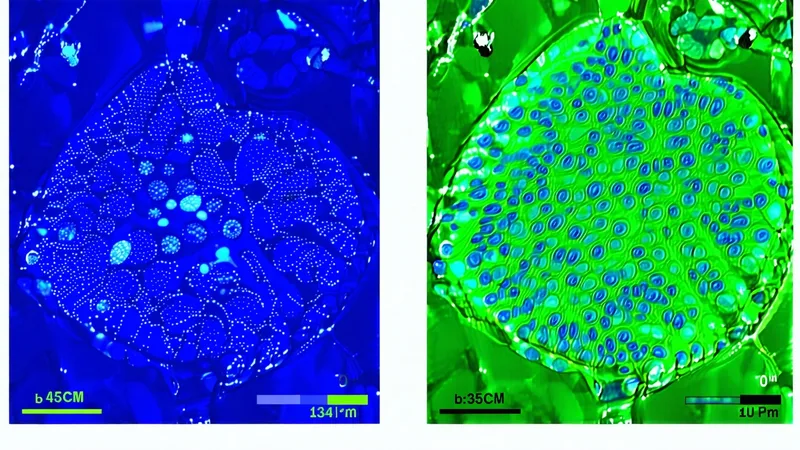
When the data are pooled for analysis, the in-house system consistently shows 25 to 40% higher mean GFP intensity in the cytoplasmic channel compared to the core facility system. The biological effect of interest — a 15% intensity shift upon compound treatment — is real but is completely obscured by the inter-site, inter-instrument offset. Neither site has done anything wrong. The variability is in the instruments.
Resolving this requires characterization of both systems with reference samples (fluorescent beads of known emission intensity, or calibrated fluorescent slides), followed by a normalization step that maps each instrument's intensity space onto a common scale. Without that step, any analysis that pools the data will be confounded.
What Does Not Fix the Problem
We are not saying that careful protocol design is unnecessary — it is essential. But protocol standardization alone does not resolve inter-instrument variability. Setting the same laser power percentage on two confocal systems does not deliver the same photon flux at the sample. Using the same camera gain setting on two sCMOS systems does not produce the same effective sensitivity. These are instrument-specific parameters, not absolute physical quantities.
Similarly, normalizing to a positive control well within a plate corrects for plate-to-plate and run-to-run variability from biological sources, but it does not correct for the optical efficiency difference between two instruments. A positive control measured on System A and a positive control measured on System B still carry the optical footprint of their respective instruments. Ratio-based normalization across channels on the same image can reduce some single-cell variability, but it does not address whole-field systematic offsets introduced by illumination non-uniformity or detector gain differences.
The Standardization Layer: What It Should Include
Reliable inter-instrument standardization requires measurements that are independent of the biology in the experiment. The practical approach involves three elements.
First, characterize illumination uniformity for each channel on each system using a fluorescent flat-field reference — either a fluorescent plastic slide or a well of sufficiently dense fluorescent solution. This produces a correction map (the flatfield image) that removes spatial intensity gradients from every subsequent biological image.
Second, measure intensity response with a calibrated reference sample — commercially available fluorescent microspheres with traceable emission values work well for this — to establish the relationship between raw detector counts and a consistent intensity unit. This calibration should be repeated at regular intervals and whenever the instrument undergoes service or objective changes.
Third, apply these corrections as a pre-processing step, before any segmentation or feature extraction occurs. Applying corrections after segmentation introduces order-of-operations errors because the thresholds used for segmentation were set on uncorrected intensity values.
The Practical Consequence for Multi-Instrument Studies
The reproducibility problem is not primarily a measurement technology problem — today's fluorescence systems are highly capable. It is a data harmonization problem. When imaging data is collected on heterogeneous instrumentation and analyzed without a systematic standardization step, quantitative comparisons between datasets are methodologically unsound even when the biology is well-controlled.
For academic labs running longitudinal studies, the implication is that images collected before and after an instrument service or objective replacement are not directly comparable without re-calibration. For drug discovery teams running HCS campaigns across multiple imaging systems, the implication is that hit calling thresholds derived on one system may generate unacceptably high false negative or false positive rates on another.
The field has long accepted this variability as a fact of life. A more useful framing is that it is a problem with a known structure and tractable solutions — provided the standardization step is built into the pipeline from the start, rather than treated as an optional post-hoc correction.
Instrument performance documentation, regular calibration with reference materials, and pre-analysis flatfield and intensity normalization are not exotic requirements. They are the minimum necessary conditions for quantitative fluorescence measurements to carry the meaning we claim they carry.